Load Project

Load and visualize an OMF project file

# sphinx_gallery_thumbnail_number = 3
import pyvista as pv

import omfvista

Load the project into an pyvista.MultiBlock dataset

project = omfvista.load_project("../assets/test_file.omf")
print(project)

MultiBlock (0x7fce466631c0)
  N Blocks    9
  X Bounds    443941.105, 447059.611
  Y Bounds    491941.536, 495059.859
  Z Bounds    2330.000, 3555.942

Once the data is loaded as a pyvista.MultiBlock dataset from omfvista, then that object can be directly used for interactive 3D visualization from pyvista:

project.plot()

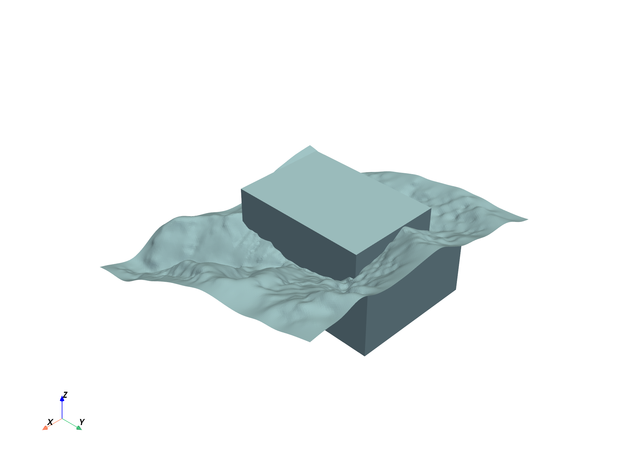
Or an interactive scene can be created and manipulated to create a compelling figure directly in a Jupyter notebook. First, grab the elements from the project:

# Grab a few elements of interest and plot em up!
vol = project["Block Model"]
assay = project["wolfpass_WP_assay"]
topo = project["Topography"]
dacite = project["Dacite"]

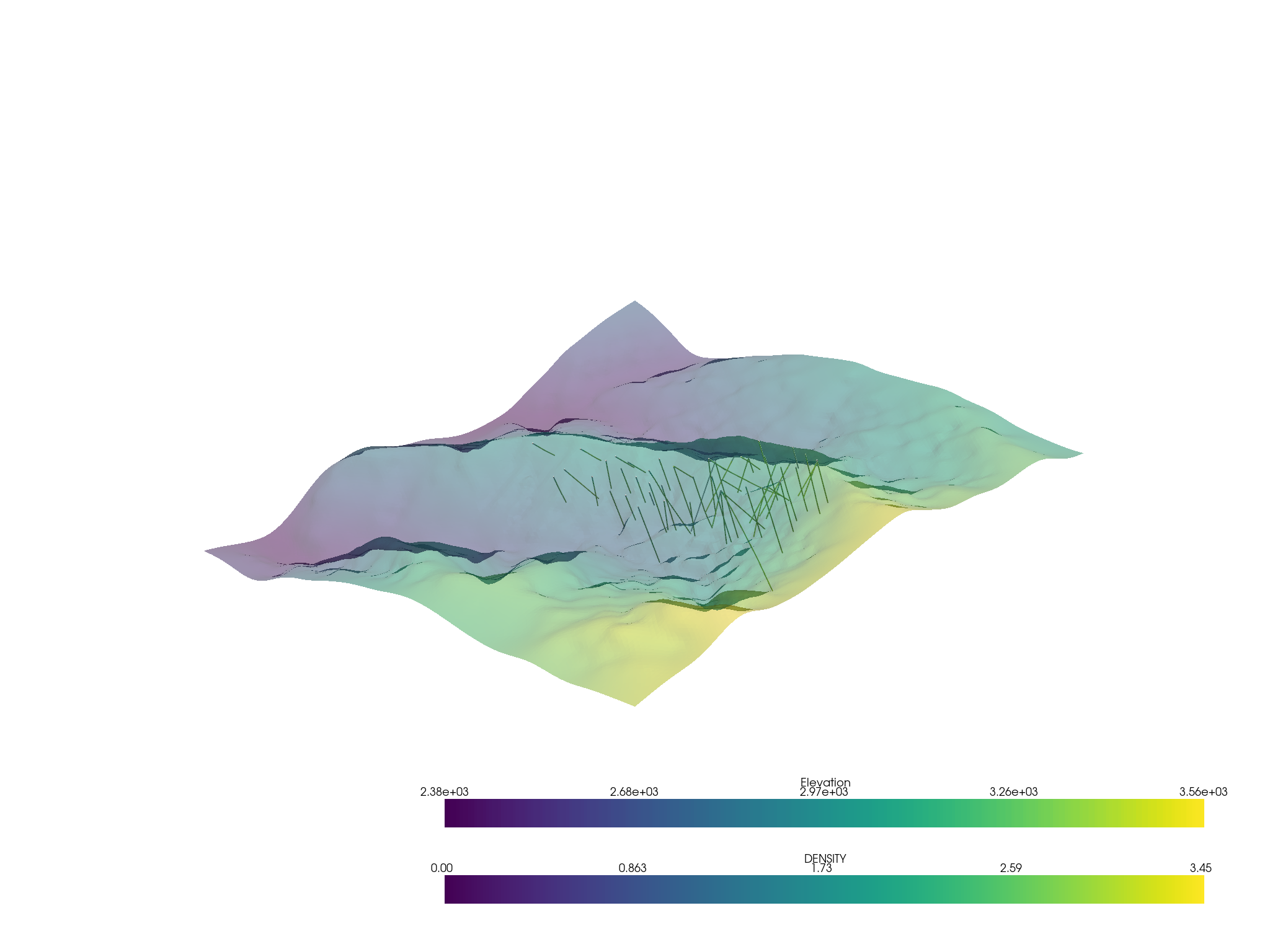
assay.set_active_scalars("DENSITY")

p = pv.Plotter()
p.add_mesh(assay.tube(radius=3))
p.add_mesh(topo, opacity=0.5)
p.show()

Then apply a filtering tool from pyvista to the volumetric data:

# Threshold the volumetric data
thresh_vol = vol.threshold([1.09, 4.20])
print(thresh_vol)

UnstructuredGrid (0x7fce466af6a0)
  N Cells:    92525
  N Points:   107807
  X Bounds:   4.447e+05, 4.457e+05
  Y Bounds:   4.929e+05, 4.942e+05
  Z Bounds:   2.330e+03, 3.110e+03
  N Arrays:   1

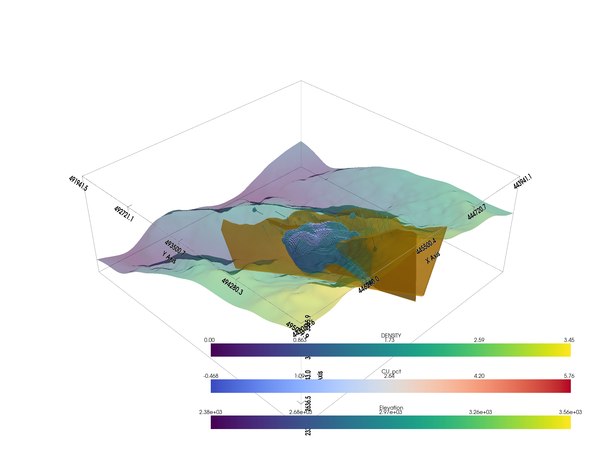
Then you can put it all in one environment!

# Create a plotting window
p = pv.Plotter()
# Add the bounds axis
p.show_bounds()
p.add_bounding_box()

# Add our datasets
p.add_mesh(topo, opacity=0.5)
p.add_mesh(
    dacite,
    color="orange",
    opacity=0.6,
)
p.add_mesh(thresh_vol, cmap="coolwarm", clim=vol.get_data_range())

# Add the assay logs: use a tube filter that varius the radius by an attribute
p.add_mesh(assay.tube(radius=3), cmap="viridis")

p.show()